REU Research Groups for Summer 2018
Descriptions of the three research groups are given below.
Statistics: Developing a Bayesian procedure to detect breakpoints in time series
Professor Jeff Liebner
A time series, as its name might suggest, is a set of observations, each one being recorded at a specific point in time. Examples include the daily closing value of the stock market, the amount of carbon dioxide at Mauna Loa on the first day of each month, or the number of children born on each day at a given hospital. These examples are just a few of the cases where such data would be encountered, so developing techniques to handle data of this nature has always been important. A particular challenge is the fact that it is fair to assume that successive observations may be related to each other. Many statistical analyses assume that data points are independent of each other, so the correlation present in time series must be accounted for. One of the most common models for describing time series is the auto-regression moving average (ARMA).
An additional challenge to fitting a time series model is the fact that the structure of the model might change in response to outside factors. While it’s easier to assume that the same model holds for all your data, this is often not realistic. The Federal Reserve could take an action that changes how stocks are traded. Sudden implementation of laws against the emission of carbon dioxide could impact the changes observed at Mauna Loa. Detecting when these changes actually are reflected in the data is important to understanding how long it takes for external factors to impact a particular time series. Some tests such as the Bai-Perron test have been developed to address this issue, but other efforts have been ongoing, especially through the use of Bayesian statistics. Our project will use a Bayesian Monte Carlo Markov Chain technique to develop a method to detect the timings of changes or breakpoints in time series. This technique will explore the possible number and timings of breaks in behavior in order to develop a fuller understanding of the actual processes that direct the data around us.
Applicants should have knowledge of probability and statistics, as well as some facility with computer programming, such as experience with R, C, Python, or similar. Familiarity with Bayesian statistics and time series analysis is not required, but some understanding of linear models will be viewed favorably.
Graph Theory: Proper Connectedness and Proper Diameter
Professors Karen McCready and Kathleen Ryan
In a graph \(G\), the distance between two vertices is the length of a shortest path between them, and the diameter of \(G\) is the maximum distance between all pairs of vertices in \(G\). The concepts of distance and diameter can be generalized to edge-colored graphs by permitting only the traversal of properly colored paths, i.e., paths where no two consecutive edges have the same color. However, in order for this generalization to be valid, we must consider only those edge-colored graphs in which a properly colored path is known to exist between any pair of vertices. Such edge-colored graphs are called properly connected. Given a properly connected edge-colored graph (like those below), we can define the proper distance between any two vertices to be the length of a shortest properly colored path and the proper diameter to be the maximum proper distance between all pairs of vertices.
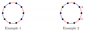
In Example 1, we see that both the proper diameter and diameter of the given cycle is 5, whereas in Example 2, the proper diameter is 8 since the shortest path between \(u\) and \(v\) is no longer properly colored and thus cannot be traversed. These examples illustrate that the diameter provides a natural lower bound for the proper diameter and that whether or not the proper diameter equals the diameter is dependent upon the given coloring. It is interesting to note that for some graphs classes, if we are constrained by the number of colors that we use, then it is impossible to find an edge-coloring in which the proper diameter equals the diameter.
This discussion and the above examples give impetus for the direction of our research group, and the following are topics of exploration to be considered: Are additional (lower and upper) bounds on the proper diameter possible? What properties of graphs and what number of colors ensure that there exists some properly connected coloring in which the proper diameter equals the diameter? How can we define a two player edge-coloring game using these notions? Along the way, our research group will also search for new properties relating to proper connectedness of edge-colored graphs.
Applicants must have completed a course in discrete mathematics. Prior knowledge of topics in graph theory, probability, and combinatorics may be helpful, but are not necessary. Some programming experience in Java, Python, or C++ may be helpful too, but is also not necessary.
Geometry: Minimal geometry in fractals
Professor Carl Hammarsten
The Cantor Set, \(\mathcal{S}\), is a famous example of a fractal, a space which exhibits interesting self-similarity across all scales. \(\mathcal{S}\) is disconnected, so paths within the set are trivial: if \(x\) and \(y\) are distinct points in \(\mathcal{S}\), there is no path from \(x\) to \(y\) that stays in \(\mathcal{S}\). When extending the definition to two dimensions, there are two distinct standard analogues of the Cantor Set: the Cantor Dust and the Sierpinski Carpet, \(\mathcal{C}\). The former is still totally disconnected and hence paths remain trivial. The latter however is actually a connected space; see the image below. Thus in \(\mathcal{C}\) one may ask about the existence and structure of geodesics, paths of minimal length joining two points. Some progress has been made on understanding these paths [e.g. Bandt and Mubarak, 2004]; but in general, and even when restricting to piecewise-linear paths, the precise answers to these questions are unknown.
In this project, we will consider taxicab paths in \(\mathcal{C}\). A taxicab path is a piecewise-linear path consisting of only horizontal and vertical segments. Specifically, we will focus on the shortest taxicab paths among triples (or larger sets) of points. By the nature of taxicab paths, it is possible that a trio of shortest paths, one for each pair of points from our triple, may have a significant amount of pairwise intersection or overlap. Can we characterize when a triple of points admits minimal paths that uniformly overlap — that is, every point on a given path is necessarily contained on a second path as well? Furthermore, for a given triple of points, if no uniformly overlapping paths exist, is there some appropriate definition of minimal “taxicab area” that they enclose? There are also natural analogues of \(\mathcal{C}\) in higher dimensions, where these questions might have interesting and necessarily different answers, and where other questions (“taxicab volumes”?) might become important.
Applicants should have completed a course in multivariable calculus and have an interest in geometry and fractals.
The picture below shows a level-4 approximation of \(\mathcal{C}\), with a level-4 approximation of \(\mathcal{S}\) highlighted in blue.